# Starbucks locations
Starbucks <- read_csv("https://jamesnormington.github.io/112_spring_2023/data/starbucks.csv")


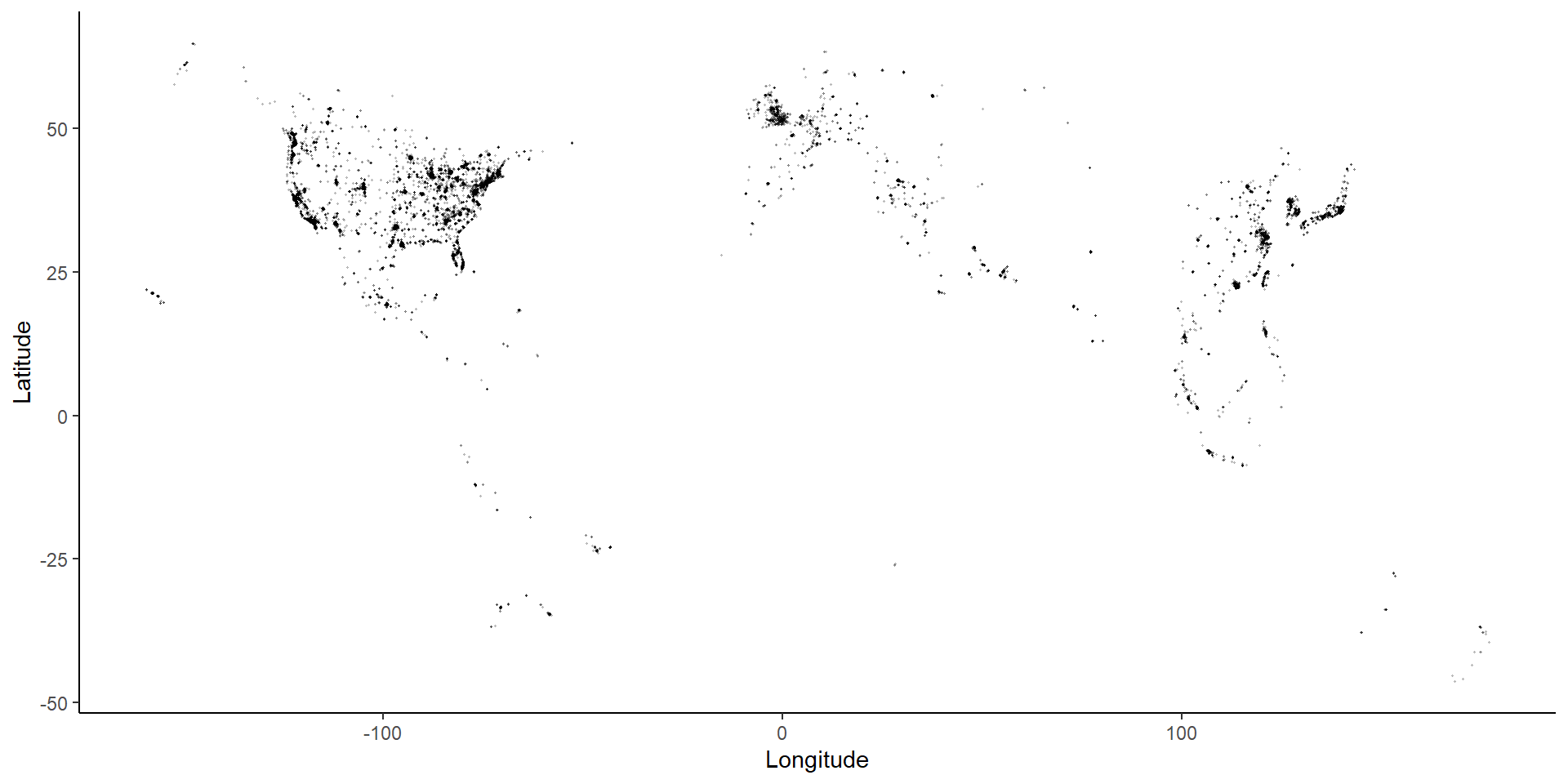
ggplot(data = Starbucks) +
  geom_point(aes(x = Longitude, y = Latitude),
    alpha = 0.2,
    size = 0.2
  ) +
  theme_classic()
ggmap() function along with ggplot2 functionsgeom_map()ggplot2 features to a map created from geom_map()leaflet, including adding points and choropleths to a base mapDownload a template .Rmd of this activity. Put the file in a Day_06 folder within your COMP_STAT_112 folder.
The Starbucks data, compiled by Danny Kaplan, contains information about every Starbucks in the world at the time the data were collected. It includes the Latitude and Longitude of each location. Let’s start by using familiar ggplot plotting tools.
# Get the map information
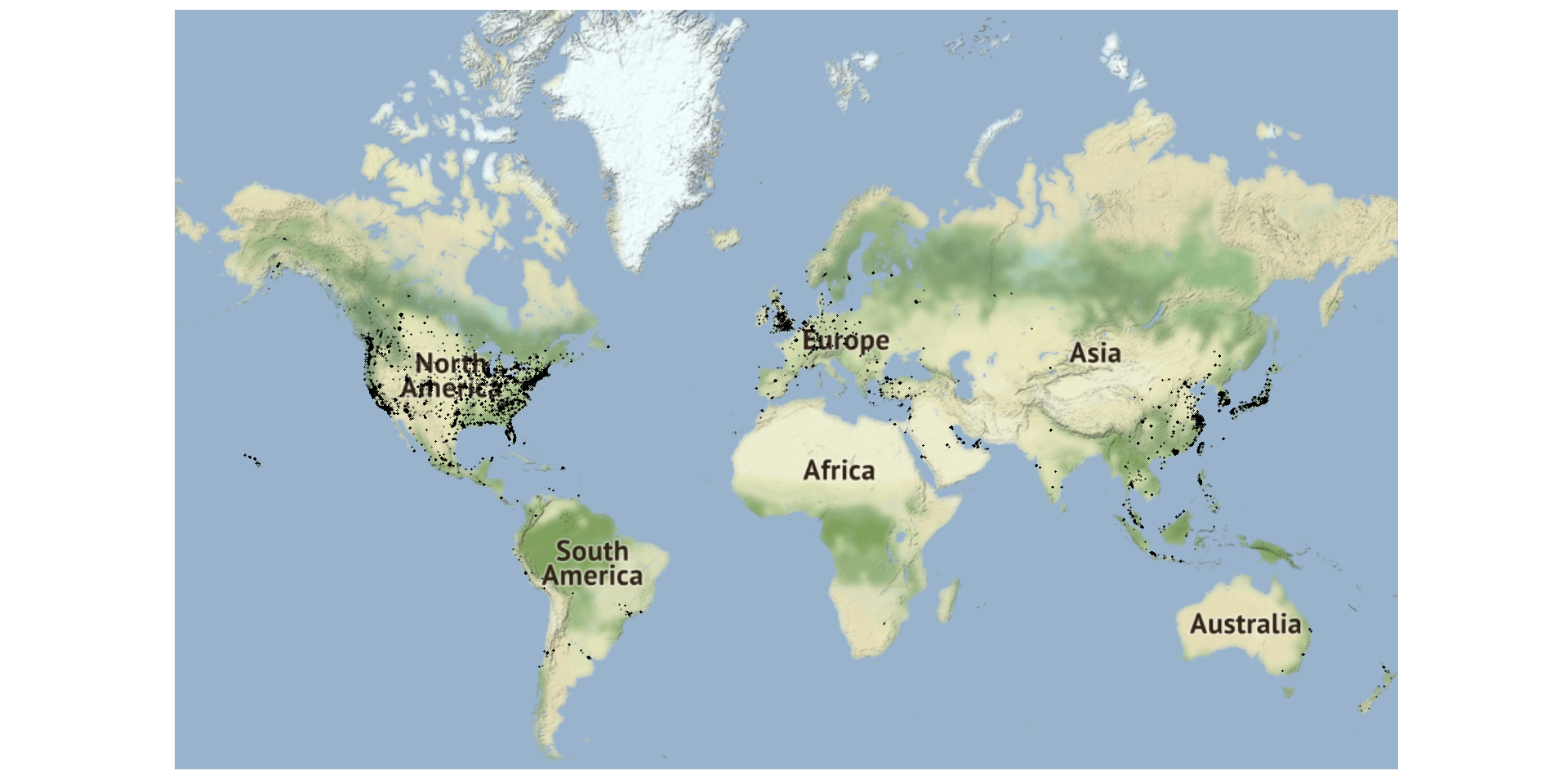
world <- get_stamenmap(
  bbox = c(left = -180, bottom = -57, right = 179, top = 82.1),
  maptype = "terrain",
  zoom = 2
)

# Plot the points on the map
ggmap(world) + # creates the map "background"
  geom_point(
    data = Starbucks,
    aes(x = Longitude, y = Latitude),
    alpha = .3,
    size = 0.2
  ) +
  theme_map()
Important Context:
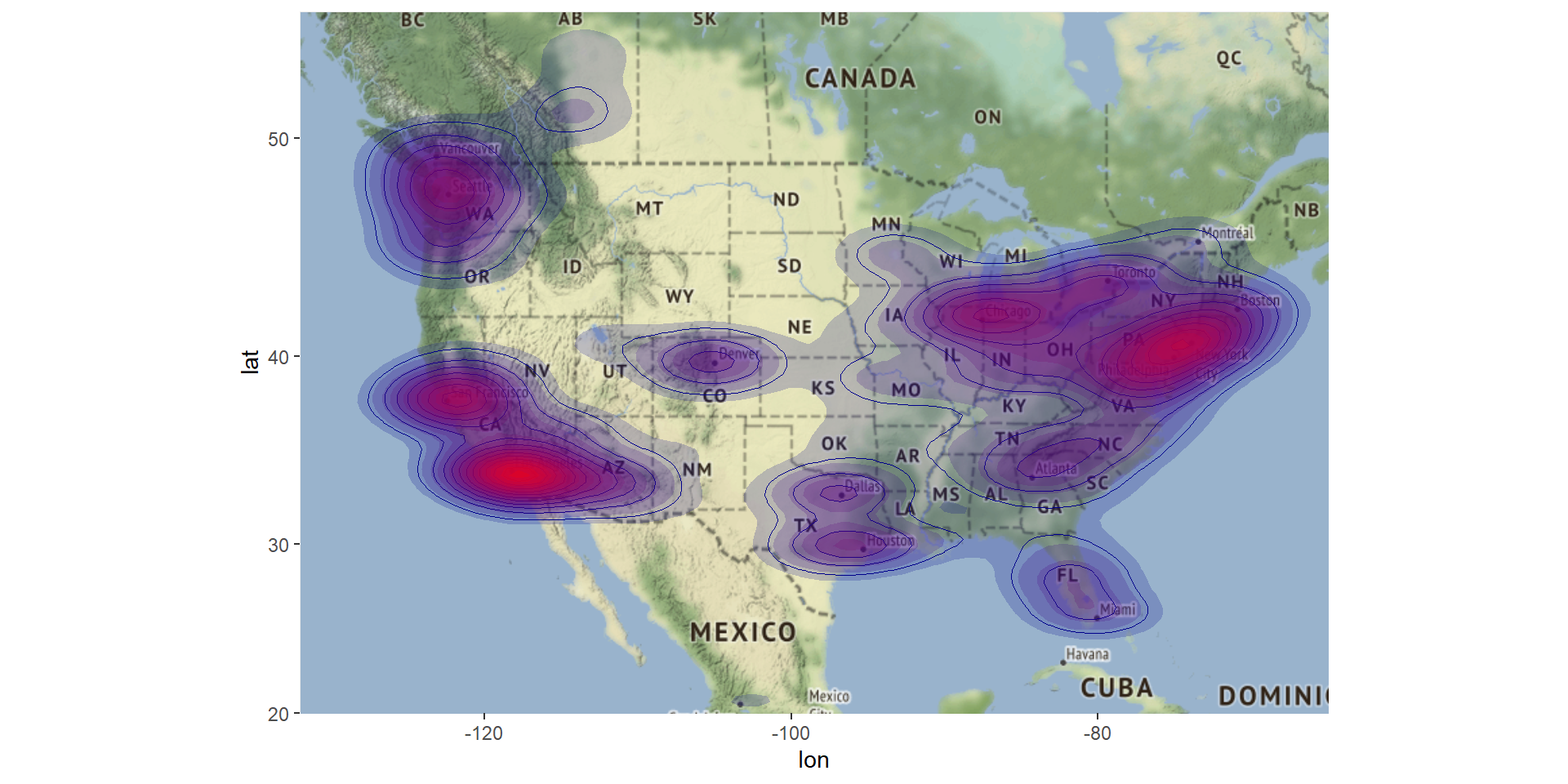
US_map2 <- get_stamenmap(
  bbox = c(left = -132, bottom = 20, right = -65, top = 55),
  maptype = "terrain",
  zoom = 4
)

ggmap(US_map2) +
  geom_density_2d(data = Starbucks, aes(x = Longitude, y = Latitude), size = 0.3, color='darkblue') +
  stat_density_2d(
    data = Starbucks,
    aes(x = Longitude, y = Latitude, fill = stat(level)),
    size = 0.1, bins = 20, geom = "polygon", alpha = 0.2
  ) +
  scale_fill_gradient(
    low = "darkblue", high = "red",
    guide = 'none'
  )
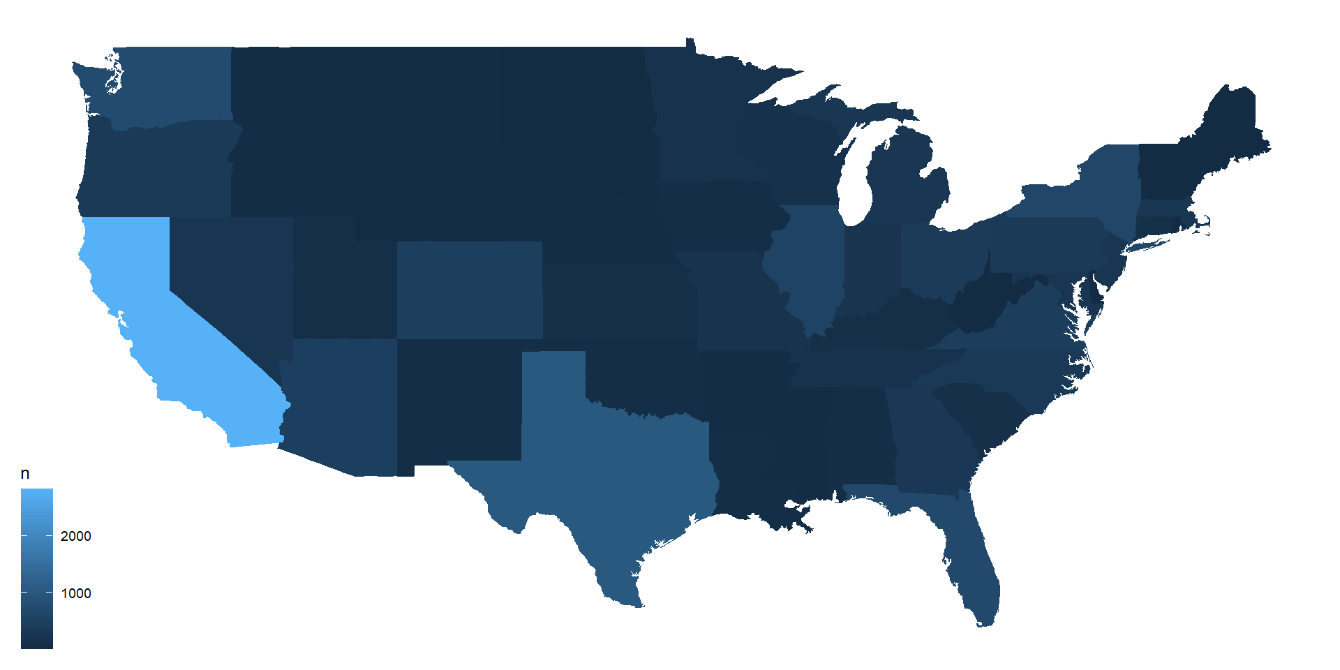
starbucks_us_by_state <- Starbucks %>%
  filter(Country == "US") %>%
  count(`State/Province`) %>%
  mutate(state_name = str_to_lower(abbr2state(`State/Province`)))

# US states map information - coordinates used to draw borders
states_map <- map_data("state")

# map that colors state by number of Starbucks
starbucks_us_by_state %>%
  ggplot() +
  geom_map(
    map = states_map,
    aes(
      map_id = state_name,
      fill = n
    )
  ) +
  # This assures the map looks decently nice:
  expand_limits(x = states_map$long, y = states_map$lat) +
  theme_map()
favorite_msp <- tibble::tibble(
  place = c(
    "Macalester College", "Stone Arch Bridge",
    "Lake Harriet", "Surly Brewing", "Boom Island Park",
    "Midtown Global Market", "Washington Ave Bridge"
  ),
  long = c(
    -93.1712321,
    -93.2534,
    -93.3062,
    -93.208633,
    -93.2687,
    -93.26054,
    -93.2393
  ),
  lat = c(
    44.9378965,
    44.9807,
    44.9222,
    44.973301,
    44.992,
    44.948780,
    44.9731
  )
)

leaflet(data = favorite_msp) %>% # base plot
  addTiles(urlTemplate = "http://{s}.tile.openstreetmap.org/{z}/{x}/{y}.png") %>% # base map - default is openstreet map
addMarkers() # Adds markers - knows lat and long from names in dataIf you want to get into spatial mapping, you’ll need to learn some GIS skills and consider coordinate reference systems (CRS).
The best tool in R to do this work is the sf package, which does work well with ggplot tools.
Assignment 4: due Wed. 2/15 @ 11:59pm
TT4 due Friday @ 11:5pm
